BenchmarkXPRT Blog banner

Tag Archives: AIXPRT

How to use alternate configuration files with AIXPRT

In last week’s AIXPRT Community Preview 3 announcement, we mentioned the new public GitHub repository that we’re using to publish AIXPRT-related information and resources. In addition to the installation readmes for each AIXPRT installation package, the repository contains a selection of alternative test config files that testers can use to quickly and easily change a test’s parameters.

As we discussed in previous blog entries about batch size, levels of precision, and number of concurrent instances, AIXPRT testers can adjust each of these key variables by editing the JSON file in the AIXPRT/Config directory. While the process is straightforward, editing each of the variables in a config file can take some time, and testers don’t always know the appropriate values for their system. To address both of these issues, we are offering a selection of alternative config files that testers can download and drop into the AIXPRT/Config directory.

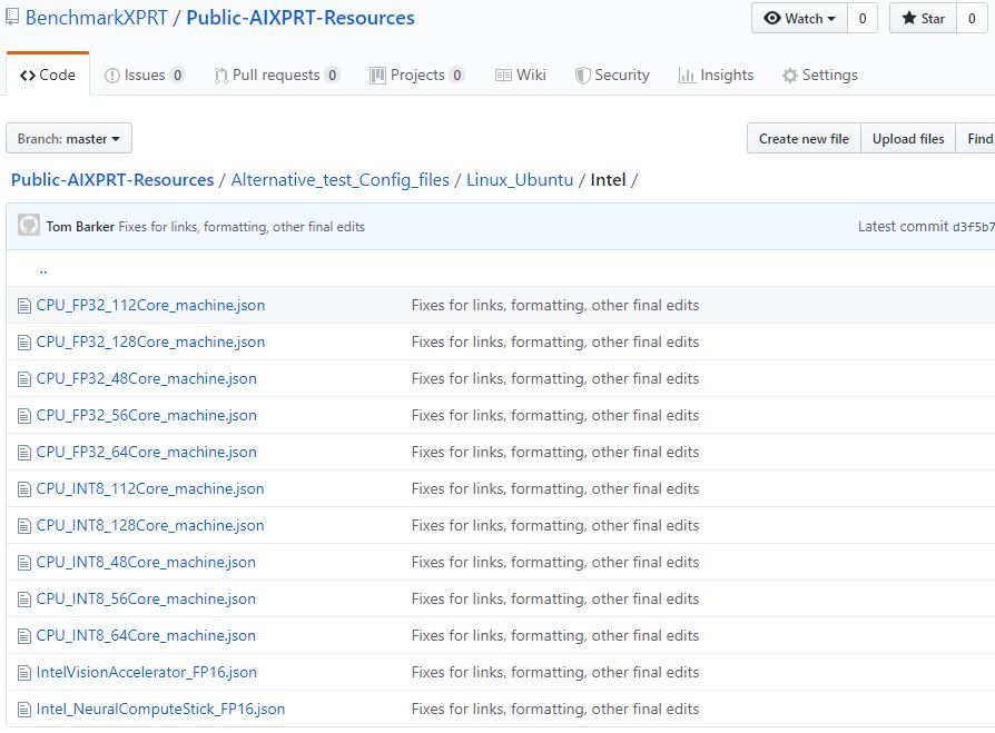
In the GitHub repository, we’ve organized the available config files first by operating system (Linux_Ubuntu and Windows) and then by vendor (All, Intel, and NVIDIA). Within each section, testers will find preconfigured JSON files set up for several scenarios, such as running with multiple concurrent instances on a system’s CPU or GPU, running with FP32 precision instead of FP16, etc. The picture below shows the preconfigured files that are currently available for systems running Ubuntu on Intel hardware.

AIXPRT public repository snip 2

Because potential AIXPRT use cases cut across a wide range of hardware segments, including desktops, edge devices, and servers, not all AIXPRT workloads and configs will be applicable to each segment. As we move towards the AIXPRT GA, we’re working to find the best way to parse out these distinctions and communicate them to end users. In many cases, the ideal combination of test configuration variables remains an open question for ongoing research. However, we hope the alternative configuration files will help by giving testers a starting place.

If you experiment with an alternative test configuration file, please note that it should replace the existing default config file. If more than one config file is present, AIXPRT will run all the configurations and generate a separate result for each. More information about the config files and detailed instructions for how to handle the files are available in the EditConfig.md document in the public repository.

We’ll continue to keep everyone up to date with AIXPRT news here in the blog. If you have any questions or comments, please let us know.

Justin

AIXPRT Community Preview 3 is here!

We’re happy to announce that the AIXPRT Community Preview 3 (CP3) is now available! As we discussed in last week’s blog, testers can expect three significant changes in AIXPRT CP3:

  • We updated support for the Ubuntu test packages from Ubuntu version 16.04 LTS to version 18.04 LTS.
  • We added TensorRT test packages for Windows and Ubuntu. Previously, AIXPRT testers could test only the TensorFlow variant of TensorRT. Now, they can use TensorRT to test systems with NVIDIA GPUs.
  • We added the Wide and Deep recommender system workload with the MXNet toolkit for Ubuntu systems.


To access AIXPRT CP3, click this access link and submit the brief information form unless you’ve already done so for CP2. You will then gain access to the AIXPRT community preview page. (If you’re not already a BenchmarkXPRT Development Community member, we’ll contact you with more information about your membership.)

On the community preview page, a download table displays the currently available AIXPRT CP3 test packages. Locate the operating system and toolkit you wish to test, and click the corresponding Download link. For detailed installation instructions and information on hardware and software requirements for each package, click the corresponding Readme link. Instead of providing installation guide PDFs as we did for CP2, we are now directing testers to a public GitHub repository. The repository contains the installation readmes for all the test packages, as well as a selection of alternative test configuration files. We’ll discuss the alternative configuration files in more detail in a future blog post.

Note: Those who have access to the existing AIXPRT GitHub repository will be able to access CP3 in the same way as previous versions.

We’ll continue to keep everyone up to date with AIXPRT news here in the blog. If you have any questions or comments, please let us know.

Justin

Understanding concurrent instances in AIXPRT

Over the past few weeks, we’ve discussed several of the key configuration variables in AIXPRT, such as batch size and level of precision. Today, we’re discussing another key variable: number of concurrent instances. In the context of machine learning inference, this refers to how many instances of the network model (ResNet-50, SSD-MobileNet, etc.) the benchmark runs simultaneously.

By default, the toolkits in AIXPRT run one instance at a time and distribute the compute load according to the characteristics of the CPU or GPU under test, as well as any relevant optimizations or accelerators in the toolkit’s reference library. By setting the number of concurrent instances to a number greater than one, a tester can use multiple CPUs or GPUs to run multiple instances of a model at the same time, usually to increase throughput.

With multiple concurrent instances, a tester can leverage additional compute resources to potentially achieve higher throughput without sacrificing latency goals.

In the current version of AIXPRT, testers can run multiple concurrent instances in the OpenVINO, TensorFlow, and TensorRT toolkits. When AIXPRT Community Preview 3 becomes available, this option will extend to the MXNet toolkit. OpenVINO and TensorRT automatically allocate hardware for each instance and don’t let users make manual adjustments. TensorFlow and MXNet require users to manually bind instances to specific hardware. (Manual hardware allocation for multiple instances is more complicated than we can cover today, so we may devote a future blog entry to that topic.)

Setting the number of concurrent instances in AIXPRT

The screenshot below shows part of a sample config file (the same one we used when we discussed batch size and precision). The value in the “concurrent instances” row indicates how many concurrent instances will be operating during the test. In this example, the number is one. To change that value, a tester simply replaces it with the desired number and saves the changes.

Config_snip

If you have any questions or comments (about concurrent instances or anything else), please feel free to contact us.

Justin

Understanding the basics of AIXPRT precision settings

A few weeks ago, we discussed one of AIXPRT’s key configuration variables, batch size. Today, we’re discussing another key variable: the level of precision. In the context of machine learning (ML) inference, the level of precision refers to the computer number format (FP32, FP16, or INT8) representing the weights (parameters) a network model uses when performing the calculations necessary for inference tasks.

Higher levels of precision for inference tasks help decrease the number of false positives and false negatives, but they can increase the amount of time, memory bandwidth, and computational power necessary to achieve accurate results. Lower levels of precision typically (but not always) enable the model to process inputs more quickly while using less memory and processing power, but they can allow a degree of inaccuracy that is unacceptable for certain real-world applications.

For example, a high level of precision may be appropriate for computer vision applications in the medical field, where the benefits of hyper-accurate object detection and classification far outweigh the benefit of saving a few milliseconds. On the other hand, a low level of precision may work well for vision-based sensors in the security industry, where alert time is critical and monitors simply need to know if an animal or a human triggered a motion-activated camera.

FP32, FP16, and INT8

In AIXPRT, we can instruct the network models to use FP32, FP16, or INT8 levels of precision:

  • FP32 refers to single-precision (32-bit) floating point format, a number format that can represent an enormous range of values with a high degree of mathematical precision. Most CPUs and GPUs handle 32-bit floating point operations very efficiently, and many programs that use neural networks, including AIXPRT, use FP32 precision by default.
  • FP16 refers to half-precision (16-bit) floating point format, a number format that uses half the number of bits as FP32 to represent a model’s parameters. FP16 is a lower level of precision than FP32, but it still provides a great enough numerical range to successfully perform many inference tasks. FP16 often requires less time than FP32, and uses less memory.
  • INT8 refers to the 8-bit integer data type. INT8 data is better suited for certain types of calculations than floating point data, but it has a relatively small numeric range compared to FP16 or FP32. Depending on the model, INT8 precision can significantly improve latency and throughput, but there may be a loss of accuracy. INT8 precision does not always trade accuracy for speed, however. Researchers have shown that a process called quantization (i.e., approximating continuous values with discrete counterparts) can enable some networks, such as ResNet-50, to run INT8 precision without any significant loss of accuracy.

Configuring precision in AIXPRT

The screenshot below shows part of a sample config file, the same sample file we used for our batch size discussion. The value in the “precision” row indicates the precision setting. This test configuration would run tests using INT8. To change the precision, a tester simply replaces that value with “fp32” or “fp16” and saves the changes.

Config_snip

Note that while decreasing the precision from FP32 to FP16 or INT8 often results in larger throughput numbers and faster inference speeds overall, this is not always the case. Many other factors can affect ML performance, including (but not limited to) the complexity of the model, the presence of specific ML optimizations for the hardware under test, and any inherent limitations of the target CPU or GPU.

As with most AI-related topics, the details of model precision are extremely complex, and it’s a hot topic in cutting edge AI research. You don’t have to be an expert, however, to understand how changing the level of precision can affect AIXPRT test results. We hope that today’s discussion helped to make the basics of precision a little clearer. If you have any questions or comments, please feel free to contact us.

Justin

Understanding AIXPRT batch size

Last week, we wrote about the basics of understanding AIXPRT results. This week, we’re discussing one of the benchmark’s key test configuration variables: batch size. Talking about batch size can be confusing, because the phrase can refer to different concepts depending on the machine learning (ML) context in which it’s used. AIXPRT tests inference, so we’ll focus on how we use batch sizes in that context. For those who are interested, we provide more information about training batch size at the bottom of this post.

Batch size in inference
In the context of ML inference, the concept of batch size is straightforward. It simply refers to the number of combined input samples (e.g., images) that the tester wants the algorithm to process simultaneously. The purpose of adjusting batch size when testing inference performance is to achieve an optimal balance between latency (speed) and throughput (the total amount processed over time).

Because of the lighter load of processing one image at a time, Batch 1 often produces the fastest latency times, and can be a good indicator of how a system handles near-real-time inference demands from client devices. Larger batch sizes (8, 16, 32, 64, or 128) can result in higher throughput on test hardware that is capable of completing more inference work in parallel. However, this increased throughput can come at the expense of latency. Running concurrent inferences via larger batch sizes is a good way to test for maximum throughput on servers.

Configuring inference batch size in AIXPRT
A good practice when trying to figure out where to start with batch size is to match the batch size to the number of cores under test (e.g., Batch 8 for eight cores). To adjust batch size in AIXPRT, testers must edit the configuration files located in AIXPRT/Config. To represent a spectrum of common tunings, AIXPRT CP2 tests Batches 1, 2, 4, 8, 16, and 32 by default.

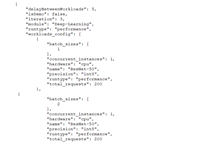
The screenshot below shows part of a sample config file. The numbers in the lines immediately below “batch_sizes” indicate the batch size. This test configuration would run tests using both Batch 1 and Batch 2. To change batch size, simply replace those numbers and save the changes.
Config_snip
Batch size in training
As we noted above, training batch size is different than inference batch size. For training, a batch is the group of samples used to train a model during one iteration and batch size is number of samples in a batch. (Note that in this context, an iteration is a single update of the algorithm’s parameters, not a complete test run.) With a batch size of one, the algorithm applies a single training sample to an image it is processing before updating its parameters. With a batch size of two, it would apply two training examples to an image before updating its parameters, and so on. Because neural network algorithms are iterative, a larger batch size setting during training increases the total number of iterations that occur during each pass through the data set. In combination with other variables, training batch size may ultimately affect metrics such as model accuracy and convergence (the point where additional training does not improve accuracy).

In the coming weeks, we’ll discuss other test configuration variables such as precision and the number of concurrent instances. We hope this series of blog entries will answer some of the common questions people have when first running the benchmark and help to make the AIXPRT testing process more approachable for testers who are just starting to explore machine learning. If you have any questions or comments, please feel free to contact us.

Justin

Understanding AIXPRT results

Last week, we discussed the changes we made to the AIXPRT Community Preview 2 (CP2) download page as part of our ongoing effort to make AIXPRT easier to use. This week, we want to discuss the basics of understanding AIXPRT results by talking about the numbers that really matter and how to access and read the actual results files.

To understand AIXPRT results at a high level, it’s important to revisit the core purpose of the benchmark. AIXPRT’s bundled toolkits measure inference latency (the speed of image processing) and throughput (the number of images processed in a given time period) for image recognition (ResNet-50) and object detection (SSD-MobileNet v1) tasks. Testers have the option of adjusting variables such as batch size (the number of input samples to process simultaneously) to try and achieve higher levels of throughput, but higher throughput can come at the expense of increased latency per task. In real-time or near real-time use cases such as performing image recognition on individual photos being captured by a camera, lower latency is important because it improves the user experience. In other cases, such as performing image recognition on a large library of photos, achieving higher throughput might be preferable; designating larger batch sizes or running concurrent instances might allow the overall workload to complete more quickly.

The dynamics of these performance tradeoffs ensure that there is no single good score for all machine learning scenarios. Some testers might prefer lower latency, while others would sacrifice latency to achieve the higher level of throughput that their use case demands.

Testers can find latency and throughput numbers for each completed run in a JSON results file in the AIXPRT/Results folder. The test also generates CSV results files that are in the same folder. The raw results files report values for each AI task configuration (e.g., ResNet-50, Batch1, on CPU). Parsing and consolidating the raw data can take some time, so we’re developing a results file parsing tool to make the job much easier.

The results parsing tool is currently available in the AIXPRT CP2 OpenVINO – Windows package, and we hope to make it available for more packages soon. Using the tool is as simple as running a single command, and detailed instructions for how to do so are in the AIXPRT OpenVINO on Windows user guide. The tool produces a summary (example below) that makes it easier to quickly identify relevant comparison points such as maximum throughput and minimum latency.

AIXPRT results summary

In addition to the summary, the tool displays the throughput and latency results for each AI task configuration tested by the benchmark. AIXPRT runs each AI task multiple times and reports the average inference throughput and corresponding latency percentiles.

AIXPRT results details

We hope that this information helps to make it easier to understand AIXPRT results. If you have any questions or comments, please feel free to contact us.

Justin

Check out the other XPRTs:

Forgot your password?